title: “Sensor Drift Correction Using Machine Learning in Online Conductivity Loops: Shanghai ChiMay Engineering Notes”
date: 2026-07-01
perspective: Technical
audience: Instrumentation Engineers, Data Scientists, Water Chemistry Specialists
keywords: sensor drift, machine learning, conductivity, drift correction, online monitoring
Table of Contents
Sensor Drift Correction Using Machine Learning in Online Conductivity Loops: Shanghai ChiMay Engineering Notes
Conductivity is one of the most widely deployed online water-quality parameters, and it is also one of the most prone to gradual measurement drift. Cell fouling, temperature-compensation error, and reference-cell aging all cause the reported conductivity value to diverge from the true water value over weeks to months. Traditional operations respond with scheduled recalibration; smart water programs are increasingly turning to machine-learning-based drift correction to close the gap between calibrations. This article describes what actually works.
Key Takeaways
- 63% of new online conductivity deployments in 2026 include some form of algorithmic drift correction, up from under 15% five years ago.
- Machine-learning drift correction typically extends the calibration interval by 1.5-2.5x without loss of measurement quality.
- Effective drift-correction models rely on contextual features — temperature, flow rate, upstream event flags — not conductivity data alone.
- Shanghai ChiMay in-line conductivity meters, electrodes, and analyzers provide the diagnostic outputs needed to feed a robust drift-correction pipeline.
The Physics of Conductivity Drift
Before applying any correction algorithm, engineers must understand the underlying drift mechanisms. Online conductivity sensors drift for several distinct reasons:
- Electrode fouling – organic films, biofilms, or mineral scale accumulate on the electrode surface and change the cell constant.
- Temperature compensation error – standard linear temperature coefficients (typically 2.0-2.1% per °C for KCl solutions) break down at low conductivities and non-KCl matrices.
- Reference cell aging – for toroidal sensors, coil impedance drifts with temperature cycling.
- Cable and connector effects – capacitive drift from long cable runs in humid environments.
Each drift source has a characteristic time signature. Fouling drifts slowly and monotonically; temperature-compensation error co-varies with process temperature; connector effects appear as step changes after weather events.
Why Statistical Methods Alone Are Not Enough
The traditional approach to drift is a scheduled recalibration every 60, 90, or 180 days. Between calibrations, most plants apply a simple rolling-average filter and hope for the best. This works, but it treats drift as a nuisance rather than a diagnostic signal. Statistical filters cannot distinguish drift from a real process change, and they cannot use context.
Machine-learning approaches offer three advantages:
- Distinction between drift and process change using contextual features.
- Predictive maintenance — the model can flag when drift acceleration warrants intervention.
- Quantified uncertainty on each reported measurement.
A Practical ML Pipeline for Drift Correction
Engineering teams looking to deploy drift correction should follow a defined pipeline:
Step 1: Feature Engineering
The model should ingest:
- Raw conductivity measurement.
- Process temperature (co-located).
- Reference cell impedance (if available).
- Upstream flow rate.
- Time since last calibration.
- Cumulative operating hours.
- Ambient temperature and humidity at the transmitter enclosure (if instrumented).
Cross-correlation analysis at the feature-engineering stage often reveals which features carry meaningful drift signal.
Step 2: Ground Truth Establishment
The model requires ground-truth data. In practice, this comes from:
- Grab-sample laboratory measurements at scheduled intervals.
- Post-calibration reference readings immediately after each field calibration.
- Redundant online instruments where deployed.
Absent labeled ground truth, unsupervised anomaly detection is the fallback, but it produces less actionable output.
Step 3: Model Selection
For conductivity drift correction, three model families work reliably:
- Gradient boosting (XGBoost, LightGBM) – strong performance on tabular features, interpretable feature importance.
- Recurrent neural networks (LSTM, GRU) – capture time-dependent drift dynamics.
- State-space and Kalman filter models – appropriate when drift physics can be parameterized.
Simpler is generally better in production. A well-tuned gradient-boosted regressor typically outperforms an LSTM on limited training data.
Step 4: Validation Discipline
Standard machine-learning validation practice applies with two water-specific twists:
- Temporal validation splits — train on early data, test on later data, never random splits.
- Process-condition stratification — hold out data from unusual operating conditions to evaluate generalization.
Step 5: Deployment and Monitoring
Deployment can be edge-side (on the transmitter or a nearby gateway) or cloud-side. Monitoring must track:
- Model residuals versus laboratory reference readings.
- Feature drift on the input side.
- Alert generation frequency.
Comparison of Drift Correction Approaches
| Approach | Calibration interval extension | Complexity | Data requirement | Best fit |
|---|---|---|---|---|
| Rolling average | 1.0x (baseline) | Very low | None | Any |
| Piecewise linear | 1.2-1.4x | Low | Regular calibration | Stable processes |
| Kalman filter | 1.4-1.8x | Medium | Physics model | Well-characterized loops |
| Gradient boosting | 1.8-2.5x | Medium | Labeled data, features | Most industrial and municipal |
| LSTM/GRU | 2.0-3.0x | High | Large labeled dataset | High-value loops with rich data |
Most water plants should start with a gradient-boosted model and only move to deep learning when the operational value clearly justifies the complexity.
Failure Modes and Guardrails
Machine-learning drift correction has real failure modes engineering teams must anticipate:
- Silent process shift — a genuine change in influent chemistry can be interpreted as drift and corrected away. Guardrail: keep the raw uncorrected value available in parallel.
- Correlated feature failure — if the temperature sensor drifts, so does the drift correction. Guardrail: monitor input features for their own drift.
- Regulatory reporting ambiguity — regulators may require the raw sensor reading, not the corrected value. Guardrail: document both values in the data historian.
Shanghai ChiMay Instrumentation Support
Shanghai ChiMay in-line conductivity meters, conductivity electrodes, and multi-parameter sensors expose the diagnostic register set typically required for drift correction pipelines: temperature, cell impedance status, and elapsed operating hours. These outputs feed directly into edge or cloud ML pipelines without additional integration effort.
Industry Outlook
By 2030, machine-learning drift correction is expected to be a standard feature on all industrial-grade online conductivity monitors. Standardization work on model performance metrics and drift-correction documentation is underway within the water instrumentation community. Engineers building smart-water programs today should insist on transparent model behavior, documented residual performance, and clean access to both raw and corrected values.
Conclusion
Machine-learning drift correction is not a magic layer that removes the need for calibration; it is a disciplined engineering practice that extends calibration intervals, provides earlier warning of sensor degradation, and improves data quality for downstream analytics. Instrumentation teams that treat drift correction as an integrated part of the measurement pipeline — not a cloud afterthought — will achieve substantially better long-term measurement quality. Shanghai ChiMay conductivity products provide the diagnostic transparency needed to make these pipelines work in real deployments.