Municipal distribution systems were historically operated half blind. Utilities knew what left the treatment plant; what happened across miles of buried pipe was largely guesswork, supported by a monthly round of pressure gauge readings and a few flow meters at pump stations. Cheap, low-power sensors and better communications have changed that. Here are the five areas where the change is most visible.
Table of Contents
1. Continuous Pressure Monitoring Prevents Catastrophic Failures
Understanding Network Pressure Dynamics
Distribution systems run under pressure — commonly in the 50–100 psi range at service connections. Below the minimum, contamination can be drawn in through joints and cracks. Above the design limit, pipe failures become a question of time rather than probability.
Most utilities used to measure pressure at pumping stations, which is exactly where problems are least likely to start. Pressure loggers at intervals along critical zones fill in the picture between those points, and that is where transient events show up.
Pressure Wave Analysis
Fast sensors capture transient events — pressure spikes and dips lasting milliseconds — caused by valve movements, pump starts and stops, or a break opening up. Those waves carry diagnostic information about the state of the network:
- Pipe wall condition, before anything shows on the surface
- Air pockets restricting flow
- Valve condition and response time
- Leak presence and approximate location
University of Exeter researchers working on transient-based detection have shown that the method can flag developing anomalies well ahead of visible failure, which is what makes it useful for replacement planning rather than just for post-mortems. The lead time depends on the pipe material, the sensor spacing and how often the network is excited by normal operations.
Pressure Monitoring Hardware
Shanghai ChiMay makes inline pressure sensors for permanent installation in distribution networks. They transmit over NB-IoT or LoRaWAN, which suits battery-powered devices spread across a large service area where running cable to each point is not realistic.
2. Smart Flow Measurement Tightens the Water Balance
Understanding Water Balance
The International Water Association (IWA) water balance is the accepted way to account for everything a utility produces:
- Authorized consumption — billed and unbilled legitimate use
- Apparent losses — metering error, unauthorized connections, data handling mistakes
- Real losses — leakage from pipes, joints and storage
Most utilities can estimate the first category. The other two are where guesswork lives, and IoT flow meters at DMA boundaries are what replace that guesswork with numbers.
District Metered Areas (DMAs)
Dividing the network into district metered areas makes loss quantification systematic. Each DMA measures:
- Inflow — total water entering the district
- Outflow — consumption recorded by service meters
- Night flow — minimum overnight use, the classic leakage indicator
Continuous metering at the boundaries allows the water balance to be recalculated daily rather than annually. DMA programs are the established route to bringing non-revenue water down; how much a utility gains depends mostly on how bad the leakage baseline is and how quickly it acts on the night-flow data.
Smart Meter Integration
Advanced metering infrastructure (AMI) brings customer meters into network optimisation:
- Automated reading, which removes the manual collection round
- Consumption pattern analysis that flags unusual use, including continuous low flow
- Prepaid options that reduce bad debt
- Demand data that sharpens supply planning
Customer-facing engagement programs built on this data have been reported to shave peak demand, though the effect depends heavily on tariff design and how the utility communicates. Treat demand reduction as a soft benefit when you build the business case.
3. Water Quality Monitoring Protects Public Health
Continuous Contamination Surveillance
Grab sampling at weekly or monthly intervals will not catch an event that lasts three hours. Continuous instruments change the detection window from weeks to minutes:
- Free chlorine residual — the primary disinfection indicator
- pH — stability and corrosion control
- Turbidity — particulates, and a proxy for pathogen risk
- Conductivity — dissolved solids and a marker of intrusion
- Dissolved oxygen — organic loading and biological activity
The operational value is not just detection. Trend data tells you whether chlorine demand is creeping up in a zone, and whether that is a seasonal temperature effect or something new in the water.
Early Warning System Architecture
A complete network usually has sensors at several levels:
- Source water — algal blooms, organic loading, chemical contamination
- Treatment processes — optimisation and failure detection
- Distribution — keeping quality stable across the network
- Point of use — verification where it matters most, such as hospitals
When an instrument alarms, the response has to be defined in advance: who is called, what sample is taken, what the fallback is. Automated alerts reduce contamination exposure — the size of the improvement depends on how complete the network is and how fast the response protocol runs.
4. Acoustic Leak Detection Pinpoints Hidden Losses
The Physics of Pipe Leaks
Water escaping from a pressurised pipe makes noise:
- High-frequency components (roughly 1–30 kHz) from turbulent flow at the leak point
- Low-frequency components (roughly 20–500 Hz) transmitted through the pipe wall and surrounding soil
- Hydrophone signals picked up through the water column
The signal travels along the pipe and can be picked up at hydrants, valves and service connections — the access points a crew can actually reach.
Correlation Technology
Leak noise correlators record the signal at two points and calculate the time difference between arrivals:
Distance = (Velocity × Time Difference) / 2
On metallic pipe in good condition, modern correlators get you within about a metre on a run of a few hundred metres. Plastic pipe is harder: the acoustic signal attenuates faster and the velocity is less predictable, so accuracy suffers and you may need more closely spaced measurement points.
Continuous Acoustic Monitoring
Fixed loggers left in the network provide 24/7 surveillance:
- Ambient noise baselines so genuine leaks stand out
- Transient analysis for intermittent leaks that only appear at certain pressures
- Magnitude estimation to prioritise the response
- Cross-correlation to confirm a location before anyone digs
The practical benefit is time. Correlation surveys used to take days to schedule and complete; permanent monitoring shortens that to a matter of hours, which matters when a leak is under a road or a hospital access.
5. Asset Management Optimization Extends Infrastructure Life
Condition-Based Maintenance
Time-based maintenance services equipment regardless of condition, which wastes money on healthy assets and misses the ones about to fail. Condition monitoring flips that:
- Vibration analysis catches bearing wear in pumps early
- Power consumption monitoring shows motor efficiency dropping
- Cycle counting supports fatigue analysis on valves and actuators
- Temperature trending points to insulation or lubrication problems
Programs built on this typically reduce unplanned failures and extend asset life, with results tracking how well the data is used rather than how many sensors were installed. Sensors with no analysis behind them do not change a maintenance program.
Risk-Based Asset Management
Not every asset deserves equal attention. Risk assessment combines:
- Probability of failure — condition, age, duty cycle, history
- Consequence of failure — service disruption, health risk, repair cost, regulatory exposure
Assets that score high on both get the inspection and replacement budget. The rest wait.
Capital Planning Integration
Operational data feeds directly into capital planning:
- Remaining useful life estimates set replacement timing
- Deterioration models project future maintenance needs
- Risk ranking allocates budget to the highest-impact projects
- Scenario analysis tests different investment strategies against each other
Utilities that run full asset management programs generally get more service life out of each capital dollar, because spending goes to the assets that need it rather than being spread evenly.
Implementation Considerations
Starting Your IoT Journey
Phase 1: Foundation
– Establish communications infrastructure
– Deploy sensors in the areas with the worst current visibility
– Stand up the data platform before scaling deployments
– Train staff on the new data and the response protocols
Phase 2: Expansion
– Extend coverage across the network
– Integrate with SCADA and asset management systems
– Bring in analytics for leak detection and pressure management
– Automate routine reporting
Phase 3: Optimization
– Move into condition-based maintenance on rotating equipment
– Apply machine learning where there is enough history to train on
– Tune operations against real consumption data
– Connect customer-facing systems for demand programs
Choosing Technology Partners
The five capabilities above only pay off if the devices stay online for years and the data is usable. When evaluating suppliers, look for:
- Proven reliability in water industry service, not just industrial credentials
- Interoperability with standard protocols, including whatever your SCADA already speaks
- Scalability from a pilot of 20 devices to a network of thousands
- Support and spares through the life of the deployment
- Integration services that connect field devices to enterprise systems
Shanghai ChiMay’s sensor range combines field-proven hardware with that support structure, which is what utilities are really buying when they move from a pilot to a full rollout.
Where This Leaves Utilities
Pressure monitoring, smart metering, continuous water quality measurement, acoustic leak detection and condition-based asset management each solve a specific operational problem. Deployed together they produce something more useful than the sum of the parts: a distribution network whose condition is visible, and whose problems are found before customers notice.
The decision is not whether to instrument the network. It is where to start, and how fast to expand once the first phase proves itself.